Bonett's (2008) Method for Confidence Intervals on Meta-Analysed Pearson's rs: Play Along in R

Yes. It's another blog about correlation coefficients. I make no apology for that. I estimate that - much like the old English adage about rats - you're never more than six feet away from a Pearson's r in personality and social psychology.

The topic at hand: confidence intervals on meta-analysed Pearson's rs. To recap, in my last blog I created an R script that would allow you to play along with Sarah's Pearson's r mini-meta analysis in the Goh, Hall, & Rosenthal (2016) paper on mini meta-analysis. After I had written that blog, I got talking to Jin on twitter about confidence intervals around meta-analysed rs.

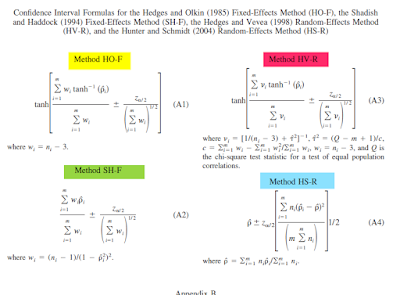
I did some digging and it turns out that there's at least 5 different methods in the literature. I know this thanks to a great paper by Professor Doug Bonnet, in which 5 methods are pitted against each other with a simulation study. It's s a kind of meta-analytic royal rumble. Which are my words, not Professor Bonnet's - I doubt that framing would have gone down well at the journal. Here's that paper, courtesy of Professor Bonnet's Researchgate.

The contenders were HO-F, SH-F, HV-R, HS-R:

And a new method proposed by Bonnet, a mysterious newcomer simply known as equation 4.

Where p hat, the unweighted average of the sample correlations, is:

Where the approximate variance of p hat is:

And where variance of tanh^-1(p hat):

To cut a story longer than is appropriate for a blog short (but read it in your own time), equation 4 comes out on top. Empirically, in terms of its performance in the simulations carried out in the paper and, logically, because it does not require a couple of unrealistic assumptions that underpin alternative methods (see page 178).

Now, I fully understand that this equation will look a little alien to some. But I have scripted it in R, so that you can play along with the computational example given on page 177. As per usual, this script can be extremely easily modified to use with your own data to create confidence intervals for your own meta-analysed rs. The script is a bit flabby I expect. People that have been coding in R longer than me will almost definitely spot some redundancy, but it get's you the desired result. Click here, or scroll to the bottom of this blog post.

All you have to do is:

• Enter your correlations in the cors <- c(.......) part.
• Enter the n for each correlation in the ns <- c(.......) part.
• Enter the number of correlations in the m <- x part.

Here's the code (thanks to Daniel Lakens for suggesting I use gist, here's his blog):

	#Confidence intervals around meta-analysed Pearson's rs
	#equation 4 from Bonett, D. G. (2008).
	#Meta-analytic interval estimation for bivariate correlations.
	#Psychological methods, 13(3), 173.
	#WHAT YOU NEED TO ENTER: Correlation coefficients (cors) and sample size (ns) for each coefficient, plus number of coefficients (m)
	#Script for following along with example on p. 177
	#input correlation coefficients
	cors <-c(.40,.65,.60,.45)
	#input sample sizes
	ns <-c(55, 190, 65, 35)
	n3 <- ns-3
	corsq <- cors*cors
	corsq2 <- 1-corsq
	corsq3 <- (corsq2)^2
	corsq4 <- corsq3/n3
	r.rc <- data.frame(cors = cors, ns = ns, n3 = n3, corsq = corsq, corsq2 = corsq2, corsq3 = corsq3, corsq4 = corsq4)
	round(r.rc,3)
	#input number of correlation coefficients HERE (m)
	m <- 4
	mmin2 <-m^-2
	#estimated variance p hat
	v <- sum(corsq4)*mmin2
	# = .00261
	#point estimate p hat (just mean average of coefficients)
	pe <-mean(cors)
	#=.525
	#get tanh-1 (p hat)
	numertan1 <- (1+pe)
	numertan2 <- (1-pe)
	numertan3 <- log(numertan1, base = exp(1))
	numertan4 <- log(numertan2, base = exp(1))
	numertan5 <- numertan3 - numertan4
	tanh1 <- numertan5/2
	tanh1
	# = .583
	#get estimated variance of tanh-1 (p hat)
	dvartanh <- (1-(pe^2))^2
	vartanh <- v/dvartanh
	vartanh
	# = .00498
	#Lower 95% confidence interval
	lci1 <- vartanh^.5
	lci2 <-1.96*lci1
	lci3 <- tanh1-lci2
	LCI <-tanh(lci3)
	LCI
	# = .41766
	#Upper 95% confidence interval
	uci1 <- vartanh^.5
	uci2 <-1.96*uci1
	uci3 <- tanh1+uci2
	UCI <-tanh(uci3)
	UCI
	# = .61788

view raw Bonnett 2008 confidence interval on meta-analysed r.R hosted with ❤ by GitHub