The MAD Method of Outlier Detection (Leys et al., 2013): Play Along in R

What is the median absolute deviation? It's the median deviation from the median for a vector of Xs, multiplied by a constant of (usually) 1.4826. What does it look like in research? Well, imagine that you're interested in extraversion in schools. It's the median difference between the extraversion score of each member of the class and the median extraversion across the class, multiplied by the magic number 1.4826. 

Working it out is straight forward. You can do it in four steps. First, find the median of a vector of Xs (median classroom extraversion score). Second, subtract this median from each X (each child's extraversion score). Third, find the median of these differences. Fourth, multiply by 1.4826.

It's good to know what the MAD is because it is the foundation of a method of outlier detection that was recently touted as a successor to, and improvement over, the standard deviation method common in psychological research (Leys, Klein, Bernard, & Licata, 2013). All you need to do after you have median standard deviation is to multiply it by 2, 2.5, or 3. Depending on how conservative you're feeling. Then add and subtract the resulting value from the median. Any Xs falling outside of this window are outliers.

In a flash report published in JESP, Leys and colleagues argue that the MAD method should be preferred to the standard deviation method. This is because the detection of outliers in the standard deviation method is heavily influenced by the presence of outliers. So using it is a bit like installing a fire alarm in your kitchen whose ability to detect a fire decreases substantially as the number of separate fires in the room increases. Which doesn't sound like a good idea.

My analogy not theirs. And I'm not even sure it's a good one, but I'll go with it for lack of any better ideas. 

Anyway. Enough of the dodgy analogies. Below is an R script for the MAD method of outlier detection for the computational example given by Leys et al. (2013). It can be easily modified for use with your own data, just change the numbers in the vector at the top, or direct it to use a column from a data frame imported in to R.

Here's the paper.

Leys, C., Klein, O., Bernard, P., & Licata, L. (2013). Detectingoutliers: Do not use standard deviation around the mean, use absolute deviationaround the median.  Journal ofExperimental Social Psychology, 49, 764-766. http://dx.doi.org/10.1016/j.jesp.2013.03.013

	#apply median absolute deviation method of outlier detection
	#for computational example provided in Ley et al. (2013)
	#Ley, C., Klein, O., Bernard, P., & Licata, L. (2013). Detecting outliers: Do not use standard deviation around the mean, use absolute deviation around the median.
	#Journal of Experimental Social Psychology, 49, 764-766. http://dx.doi.org/10.1016/j.jesp.2013.03.013
	#get targetted vector (a)
	a <- c(1, 3, 3, 6, 8, 10, 10, 1000) #change this to another vector, or a column of a data frame, to apply to your own data
	#find median
	med <- median(a)
	#subtract median from Xs
	medsub <- (a-med)
	#make positive
	medsubpos <- abs(medsub)
	#find median deviation
	meddev <- median(medsubpos)
	#multiply by 1.4826
	meddev1 <- meddev*1.4826
	#multiply this by 2, 2.5, or 3 to find decision criterion
	#--- CHOOSE ONE ----
	#3 in example
	cutoff <- meddev1*2
	cutoff <- meddev1*2.5
	cutoff <- meddev1*3 #this one in example
	#locutoff
	LC <- med - cutoff
	#hicutoff
	HC <- med + cutoff
	#find distance from decision criterion (p.3) #191.36 for 1000
	distance <- (a-med)/meddev1
	#put above information in to a data frame
	dfoutlier <- data.frame(a = a, medsub = medsub, meddev = meddev, LC = LC, HC = HC, distance = distance)
	round(dfoutlier,3)
	#take outlier out and put in to new data frame (change value in accordance with chosen decision criterion)
	df1 <- subset.data.frame(dfoutlier, distance > 3)
	#take out the outliers from data set and create new data frame
	df2 <- subset.data.frame (dfoutlier, distance < 3)

view raw gistfile1.txt hosted with ❤ by GitHub

Behind the Scenes at the Cronbach's Alpha: Variance and Covariance Methods in R

If you can't be bothered to read all of this: alpha is just total inter-item covariance divided by total score variance, multiplied by the number of items in the scale divided by the number of items in the scale minus one. So don't hang your hat on it.

Cronbach's alpha (Cronbach, 1951) needs little introduction. It's ubiquitous in personality and social psychology, as well as in neighboring disciplines. You'll see a Cronbach's alpha on most of the occasions that a multi-item self-report scale is used.

Now Cronbach's alpha first came on the scene in the early 1950s (well, technically it's a modification of pre-existing formulas, so perhaps that's a little imprecise, but whatever). Which is an era before the widespread availability of computers. Which means that the math(s) is fairly simple. Which means it can be done by hand (or by a string of simple transparent steps in R) quite easily. Because we're so used to SPSS or SAS or some other statistical program doing it for us, some might not be aware of that. I certainly wasn't until quite recently.

Alpha was designed as an index of internal consistency reliability, which is not the same thing as internal consistency or reliability per se (depending of course how you're defining those terms), although it's often interpreted as one of the two or both (which it may well be, depending on how you're defining those terms). Although it is described in a number of ways in the psychometric literature, the mathematical operation is unequivocal. In short, it tells us about the ratio of inter-item co-variance (the extent to which responses to statements or questions contained in a scale are linearly related in a sample) to total score variance (the extent to which total scores are dissimilar in a sample), taking in to account the scale length.

Because of the existence of simple associations between variances and covariances and actually even pearson's rs in psychometric data, Cronbach's alpha can be expressed in a variety of different ways. You get exactly the same result with both of the following equations, as the code at the bottom of this blog testifies to:

Where V is variance, C is covariance, and n is the number of items in the scale (not sample size, alpha his little directly to do with sample size). Note that this is the population variance, not sample variance.

I have created an R script that lets you see behind the scenes, when Cronbach's alpha is calculated using both formulas. The script is set up for an analysis of a hypothetical five item scale with hypothetical data (download the .csv here) but can be easily modified for others. All you need to do is enter your data as a .csv file and enter the number of items in the scale.

Entering the number of items in the scale manually has the added bonus of showing how alpha changes with scale length, even when the item covariance/total score variance (equation 2) or item variance/total score variance (equation 1) stays the same. This demonstrates how gross features of the covariance-variance matrix can be identical, but differential scale length results in different alpha coefficients.

Below is the equation in the SPSS documentation. Slightly different notation is used, but the equation corresponds to the first expression of alpha in terms of summed variances of items.

	#Under the Bonnet of Cronbach's alpha.
	#COVARIANCE METHOD*
	#n/(n-1)*(sumsumCij/Vt)
	#import csv
	df1 <- read.csv("Cron.csv")
	#create cov-var matrix: 5 variances on diagonal, 20 covariances in symettric matrix (10 above, 10 below diagonal)
	cvmatrx <- cov(df1)
	#put the rows and columns of cov matrix in to a vector
	cvmatrx2 <- cvmatrx[1:25]
	#and sum
	totalvar <- sum(cvmatrx2)
	#for total of covariance-variance matrix *denominator*
	#(which is equivalent to the sample variance of total test scores)
	#sum rows (10 values in 5*5 matrix)
	sumrows <- cvmatrx[2] + cvmatrx[3] + cvmatrx[4] + cvmatrx [5] + cvmatrx [8] + cvmatrx [9] + cvmatrx [10] + cvmatrx[14] + cvmatrx[15] + cvmatrx [20]
	#sum columns (10 values in 5*5 matrix)
	sumcols <- cvmatrx[6] + cvmatrx[11] + cvmatrx[12] + cvmatrx [16] + cvmatrx [17] + cvmatrx [18] + cvmatrx [21] + cvmatrx[22] + cvmatrx[23] + cvmatrx [24]
	#check both figures are the same
	#and sum
	numerator <- sumrows+sumcols
	#find ratio of inter-item covariance to total test score variance
	ratio <- (numerator/totalvar)
	#enter number of items
	n <- 5 #enter here. Note n is number of items not sample size in Cronbach's notation
	#Change the number of items to see how under the same covariance conditions, Cronbach's alpha "improves"
	#as scale length increases
	#create multiplier
	multiplier <- n/(n-1)
	#Find alpha *ITEM COVARIANCE METHOD*
	cronbachalpha <- multiplier*(numerator/totalvar)
	#with .csv given = .334821
	#*VARIANCE METHOD*
	#(***population variance*** not sample variance - R var() in stats package is sample variance and has no
	#population variance function. Why?!)
	#get item variance
	itemvar <- var(df1$X1) + var(df1$X2) + var(df1$X3) + var(df1$X4) + var(df1$X5)
	#convert to population, differs by a factor of (n-1)/n (where n is sample size)
	#already have n, so nn will be sample size
	nn <- 10
	#get pop variance
	itemvarp <- itemvar*((nn-1)/nn)
	#get total score variance
	totalscores <- df1$X1 + df1$X2 + df1$X3 + df1$X4 + df1$X5
	#Get variance
	totalvar <- var(totalscores)
	#convert to population var
	totalvarp <- totalvar*((nn-1)/nn)
	#find item variance over total score variance, subtracted from 1
	ivtsv1 <- 1-(itemvarp/totalvarp)
	#find alpha
	cronbachalpha2 <- multiplier*ivtsv1
	#check the same

view raw Cronbach script 2102.R hosted with ❤ by GitHub

Test Contrasts Among a Set of Correlated Correlations (Meng, Rosenthal, & Rubin, 1992, using equation 6): Play along in R

Imagine for a moment that your research involves many participants, each measured on an array of predictor variables and a focal criterion variable. Imagine that, working in exploratory mode, you correlate each variable with the focal criterion variable. After you do this, you want to know whether one of the variables is more strongly associated with the criterion than the others - or a number of others. Alternatively, imagine that, working in confirmatory mode, you have a theory that predicts one variable will be more strongly associated with the criterion variable than the others.

How do you go about testing either of these things? Well, thanks to Meng, Rosenthal, and Rubin (1992), you might do it by testing contrasts among a set of correlated correlations with the following equation:

Where the upside down y is contrast weight for each X, the zr is the fisher's z transform for X on Y, rx is the median inter-correlation between Xs, and h is found by equations 2 and 3. So the full thing boils down to three equations:

We can use the code from my previous blog to find h. So that's sorted. It's just the rest we need to worry about.

The following code allows you to play along with the example in the paper. As per usual, it can be very easily modified to use with you own data. Just plug in your own coefficients, the N, and median inter-correlation. Then plug in the your contrast weights in the second step. Important: As with most of the R scripts on this blog, it wont work if the psych package is not installed and loaded.

So did you want to test whether one thing you're interested in is correlated with something to a greater or lesser extent than a bunch of other things? You can do that with this method.

	#Testing a Contrast Among CORRELATED correlation coefficients as in Meng et al. (1992).
	#Meng, X. L., Rosenthal, R., & Rubin, D. B. (1992).
	#Comparing correlated correlation coefficients. Psychological bulletin, 111(1), 172.
	#http://psycnet.apa.org/journals/bul/111/1/172/
	#ABSTRACT
	#Provides simple but accurate methods for comparing correlation coefficients between a dependent variable and
	#a set of independent variables. The methods are simple extensions of O. J. Dunn and V. A. Clark's (1969) work
	#using the Fisher z transformation and include a test and confidence interval for comparing 2 correlated
	#correlations, a test for heterogeneity, and a test and confidence interval for a contrast among
	#k (>2) correlated correlations. Also briefly discussed is why the traditional Hotelling's t test
	#for comparing correlations is generally not appropriate in practice.
	#The following code is based on equations 2, 3, 5. and 6. Allows the user to perform heterogeneity test
	# of k correlated coefficients and contrast among them. Useful when theory dictates that correlations
	#should be non-uniform and when theory dictates some should be less/more strongly correlated with
	#a dependent variable
	#Contrast test involves two steps. The first, we have to find h. This is done using the test of heterogeneity.
	#The second is the contrast test itself. The following code consists of the first and second steps.
	#STEP 1 -- STEP 1 -- STEP 1 -- STEP 1 -- STEP 1 -- STEP 1 --
	#The method of finding h is as follows. Start coefficients, ns and median intercorrelations,
	#are those in the computational examples given in this paper.
	#Replace for own data, changing coefficients, n, median intercorrelation, contrast weights as appropriate.
	#This part creates a table containing the data we will need for later computations
	cors <- c(.63, .53, .54, -.03) # put correlation coefficients (Xs -> Y) in here
	zs <- fisherz(cors) #fisherz transforms
	rs <- fisherz2r(zs) #transformations back
	round(zs,2)
	mz <- mean(zs) #mean fisher z
	zmz <- zs-mz #fisher z minus mean fisher z
	zmz2 <- zmz*zmz #fisher z minus mean fisher z squared
	cw <- c(1, 1, 1, -3) #put contrast weights in here, presently 3 to 1
	cwzs <- cw*zs #contrast weights multiplied by fisher z
	cw2 <-cw^2 #contrast weight square
	n <- 15 #n - put n here
	r <- c(.63, .53, .54, -.03) # put correlation coefficients (Xs -> Y) in here
	rc <- matrix(r.con(r,n),ncol=2) #confidence intervals of r
	t <- r*sqrt(n-2)/sqrt(1-r^2) #t
	p <- (1-pt(t,n-2))/2 #p
	square <-r*r #r squared
	r.rc <- data.frame(r=r,z=fisherz(r),lower=rc[,1],upper=rc[,2],t=t,p=p,rsquare=square,zmz=zmz, zmz2 = zmz2, cw=cw, cwzs=cwzs, cw2=cw2)
	round(r.rc,3) #creates data frame r.rc
	#average r square
	avrsqur <- mean(square)
	#sum of fishers z- mean fishers z
	sumzmz <- sum(zmz2)
	#enter median intercorrelation of Xs
	mi <- (.37) # INPUT MEDIAN CORRELATION HERE
	#find f
	f <- (1-mi)/(2*(1-avrsqur))
	f
	#0.4158828, .4159 to 2dp as given in example
	#find h
	h <- (1-(f*avrsqur))/(1-avrsqur)
	h
	#1.187071, 1.1871 to 2dp as given in example
	#find chi-square (k-1) # THIS CHI-SQUARE IS A TEST OF THE HETEROGENEITY OF THE CORRELATED COEFFICIENTS
	chisqu1 <- (n-3)*sumzmz
	chisqu2 <- (1-mi)*h
	chisqu <- chisqu1/chisqu2
	chisqu
	# 5.711426
	#FIND P for CHISQU = statistic and df
	pchisq(chisqu,3, lower.tail=FALSE)
	#STEP 2 -- STEP 2 -- STEP 2 -- STEP 2 -- STEP 2 -- STEP 2
	#we know have chi-square and h, success! We need to take h an do some other stuff with it for our contrast test.
	scwzs <- sum(cwzs) #sum of contrast weights fisher z transform (first part of test) #2.025 in example
	denom1 <- sum(cw2) #sum of contrast weights squared
	denom2 <- 1 - mi #1 - median intercorrelation of X's
	ct1 <- (n-3)/ (denom1*denom2*h)
	ct2 <- sqrt(ct1)
	contrastz <- scwzs*ct2
	#PRINT Z FOR CONTRAST, THIS IS YOUR Z TEST FOR CONTRAST AMONG CORRELATED CORRELATION COEFFICIENTS.
	contrastz
	# in Mengs example = 2.34 (2dp)
	#FIND one-tailed p for z
	pnorm(-abs(contrastz))
	#Created by Adam Pegler, 10.02.2017, email adamjpegler@gmail.com for questions, comments or complaints

view raw contrast of correlated coefficients from meng 1992 r script.R hosted with ❤ by GitHub

Bonett's (2008) Method for Confidence Intervals on Meta-Analysed Pearson's rs: Play Along in R

Yes. It's another blog about correlation coefficients. I make no apology for that. I estimate that - much like the old English adage about rats - you're never more than six feet away from a Pearson's r in personality and social psychology.

The topic at hand: confidence intervals on meta-analysed Pearson's rs. To recap, in my last blog I created an R script that would allow you to play along with Sarah's Pearson's r mini-meta analysis in the Goh, Hall, & Rosenthal (2016) paper on mini meta-analysis. After I had written that blog, I got talking to Jin on twitter about confidence intervals around meta-analysed rs.

I did some digging and it turns out that there's at least 5 different methods in the literature. I know this thanks to a great paper by Professor Doug Bonnet, in which 5 methods are pitted against each other with a simulation study. It's s a kind of meta-analytic royal rumble. Which are my words, not Professor Bonnet's - I doubt that framing would have gone down well at the journal. Here's that paper, courtesy of Professor Bonnet's Researchgate.

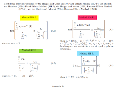
The contenders were HO-F, SH-F, HV-R, HS-R:

And a new method proposed by Bonnet, a mysterious newcomer simply known as equation 4.

Where p hat, the unweighted average of the sample correlations, is:

Where the approximate variance of p hat is:

And where variance of tanh^-1(p hat):

To cut a story longer than is appropriate for a blog short (but read it in your own time), equation 4 comes out on top. Empirically, in terms of its performance in the simulations carried out in the paper and, logically, because it does not require a couple of unrealistic assumptions that underpin alternative methods (see page 178).

Now, I fully understand that this equation will look a little alien to some. But I have scripted it in R, so that you can play along with the computational example given on page 177. As per usual, this script can be extremely easily modified to use with your own data to create confidence intervals for your own meta-analysed rs. The script is a bit flabby I expect. People that have been coding in R longer than me will almost definitely spot some redundancy, but it get's you the desired result. Click here, or scroll to the bottom of this blog post.

All you have to do is:

• Enter your correlations in the cors <- c(.......) part.
• Enter the n for each correlation in the ns <- c(.......) part.
• Enter the number of correlations in the m <- x part.

Here's the code (thanks to Daniel Lakens for suggesting I use gist, here's his blog):

	#Confidence intervals around meta-analysed Pearson's rs
	#equation 4 from Bonett, D. G. (2008).
	#Meta-analytic interval estimation for bivariate correlations.
	#Psychological methods, 13(3), 173.
	#WHAT YOU NEED TO ENTER: Correlation coefficients (cors) and sample size (ns) for each coefficient, plus number of coefficients (m)
	#Script for following along with example on p. 177
	#input correlation coefficients
	cors <-c(.40,.65,.60,.45)
	#input sample sizes
	ns <-c(55, 190, 65, 35)
	n3 <- ns-3
	corsq <- cors*cors
	corsq2 <- 1-corsq
	corsq3 <- (corsq2)^2
	corsq4 <- corsq3/n3
	r.rc <- data.frame(cors = cors, ns = ns, n3 = n3, corsq = corsq, corsq2 = corsq2, corsq3 = corsq3, corsq4 = corsq4)
	round(r.rc,3)
	#input number of correlation coefficients HERE (m)
	m <- 4
	mmin2 <-m^-2
	#estimated variance p hat
	v <- sum(corsq4)*mmin2
	# = .00261
	#point estimate p hat (just mean average of coefficients)
	pe <-mean(cors)
	#=.525
	#get tanh-1 (p hat)
	numertan1 <- (1+pe)
	numertan2 <- (1-pe)
	numertan3 <- log(numertan1, base = exp(1))
	numertan4 <- log(numertan2, base = exp(1))
	numertan5 <- numertan3 - numertan4
	tanh1 <- numertan5/2
	tanh1
	# = .583
	#get estimated variance of tanh-1 (p hat)
	dvartanh <- (1-(pe^2))^2
	vartanh <- v/dvartanh
	vartanh
	# = .00498
	#Lower 95% confidence interval
	lci1 <- vartanh^.5
	lci2 <-1.96*lci1
	lci3 <- tanh1-lci2
	LCI <-tanh(lci3)
	LCI
	# = .41766
	#Upper 95% confidence interval
	uci1 <- vartanh^.5
	uci2 <-1.96*uci1
	uci3 <- tanh1+uci2
	UCI <-tanh(uci3)
	UCI
	# = .61788

view raw Bonnett 2008 confidence interval on meta-analysed r.R hosted with ❤ by GitHub

Sarah's Pearson's r mini-meta analysis (Goh, Hall, & Rosenthal, 2016): Play along and modify for your data in R

There's this really great paper by Jin Goh and colleagues about mini meta-analyses. The idea is that in multiple study papers (and I'm thinking also multiple sample papers) it is a good idea to combine research results at some point. It's a good idea for a number of reasons, including: to subvert the p-hack culture, to help power analyses in future research, to find effects that are only observable across multiple studies (presumably due to moderator effects), and to provide stronger evidence of null findings. Get the pdf here.

I'm a social and/or personality psychology phd student with a penchant for the psychometric side of things, so I'm most interested in mini meta-analyses of Pearson's rs. You can't move for rs in my line of work. So I was naturally particularly interested in the weighted mean correlation mini meta method described on page 542 and demonstrated in an example on page 539.

This is Sarah's data:

Jin has an excel file that accompanies the paper that you can download. I have created an R script which allows you to arrive at the weighted mean correlations (fisher's z and converted back to r). You can download it here from my dropbox. It will allow you to play along with the example given by Goh and colleagues. It can be extremely easily modified to use on your own data - whenever you have comparable Pearson's r across studies or samples! Which is really probably 70% of the time.

This is what it looks like, it's really a simple thing. Just plug your own coefficients in to the cors <- c(.05, .40), taking out the original coefficients and extending the vector as long as you need it to be. Just separate coefficients by commas. And also plug your own study or sample N  in to the n <- c(80, 200) part. It is contingent on the psych package being installed and loaded, so make sure that is the case!

So, go forth and mini meta-analyse!

Here's the reference for the paper:

Goh, J. X., Hall, J. A., & Rosenthal, R. (2016). Mini Meta‐Analysis of Your Own Studies: Some Arguments on Why and a Primer on How. Social and Personality Psychology Compass, 10(10), 535-549.

And here's the code from Gist:

	#Weighted r mini meta-analysis from Goh, Hall, & Rosenthal (2016) p. 542
	#Mini Meta-Analysis of Your Own Studies: Some Arguments on Why and a Primer on How
	#Social and Personality Psychology Compass 10/10 (2016), 535-549, 10.1111/spc3.12267
	#Sarah's data example Table 2, p. 539, Agreeableness
	#do transformations and find n-3 and n3*zs
	cors <- c(.05, .40)
	n <- c(80, 200)
	zs <- fisherz(cors)
	n3 <- n-3
	n3z <- n3*zs
	r.rc <- data.frame(cors = cors,zs = zs, n3 = n3, n3z = n3z)
	#calculate rz
	#step 1
	numer <-sum(n3z)
	#step 2
	denom <-sum(n3)
	#step 3
	rz <- numer/denom
	#print statistic
	rz
	#Convert back to r
	fisherz2r(rz)
	#Sarah's data example Table 2, p. 539, Conscientiousness
	#do transformations and find n-3 and n3*zs
	cors <- c(.17, .38)
	n <- c(80, 200)
	zs <- fisherz(cors)
	n3 <- n-3
	n3z <- n3*zs
	r.rc <- data.frame(cors = cors,zs = zs, n3 = n3, n3z = n3z)
	#calculate rz
	#step 1
	numer <-sum(n3z)
	#step 2
	denom <-sum(n3)
	#step 3
	rz <- numer/denom
	#print statistic
	rz
	#Convert back to r
	fisherz2r(rz)
	#Sarah's data example Table 2, p. 539, Extraversion
	#do transformations and find n-3 and n3*zs
	cors <- c(.17, .24)
	n <- c(80, 200)
	zs <- fisherz(cors)
	n3 <- n-3
	n3z <- n3*zs
	r.rc <- data.frame(cors = cors,zs = zs, n3 = n3, n3z = n3z)
	#calculate rz
	#step 1
	numer <-sum(n3z)
	#step 2
	denom <-sum(n3)
	#step 3
	rz <- numer/denom
	#print statistic
	rz
	#Convert back to r
	fisherz2r(rz)
	#Sarah's data example Table 2, p. 539, Openess
	#do transformations and find n-3 and n3*zs
	cors <- c(.04, -.19)
	n <- c(80, 200)
	zs <- fisherz(cors)
	n3 <- n-3
	n3z <- n3*zs
	r.rc <- data.frame(cors = cors,zs = zs, n3 = n3, n3z = n3z)
	#calculate rz
	#step 1
	numer <-sum(n3z)
	#step 2
	denom <-sum(n3)
	#step 3
	rz <- numer/denom
	#print statistic
	rz
	#Convert back to r
	fisherz2r(rz)
	#Sarah's data example Table 2, p. 539, Neuroticism
	#do transformations and find n-3 and n3*zs
	cors <- c(.32, .50)
	n <- c(80, 200)
	zs <- fisherz(cors)
	n3 <- n-3
	n3z <- n3*zs
	r.rc <- data.frame(cors = cors,zs = zs, n3 = n3, n3z = n3z)
	#calculate rz
	#step 1
	numer <-sum(n3z)
	#step 2
	denom <-sum(n3)
	#step 3
	rz <- numer/denom
	#print statistic
	rz
	#Convert back to r
	fisherz2r(rz)

view raw pearsons r mini meta script for Goh et al 2016.R hosted with ❤ by GitHub